Predictive Modeling with Linear Regression
Linear regression is a popular machine learning algorithm used for predicting continuous numerical values. It is a statistical approach to modelling the relationship between a dependent variable and one or more independent variables. In this blog post, we will discuss the working of linear regression, its assumptions, and the different types of linear regression.

Working of linear Regression :
The basic idea behind linear regression is to find the line of best fit between the independent and dependent variables. This line of best fit is also known as the regression line. It is represented by the equation y = mx + b, where y is the dependent variable, x is the independent variable, m is the slope of the line, and b is the y-intercept.
The algorithm works by first plotting the data on a scatter plot to visualize the relationship between the two variables. The goal is to find a line that minimizes the distance between the predicted values and the actual values. This is done by minimizing the sum of the squared residuals.
The residuals are the differences between the predicted values and the actual values. The sum of the squared residuals is minimized using the method of least squares. This involves finding the values of m and b that minimize the sum of the squared residuals.
Assumptions :
There are several assumptions that are made in linear regression. These assumptions are important because violating them can lead to inaccurate predictions. The assumptions are as follows:
Linearity: There should be a linear relationship between the dependent and independent variables.
Independence: The observations should be independent of each other.
Homoscedasticity: The variance of the residuals should be constant across all levels of the independent variable.
Normality: The residuals should be normally distributed.
No multicollinearity: The independent variables should not be highly correlated with each other.
Types of linear regression:
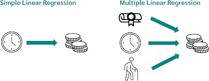
There are two types of linear regression: simple linear regression and multiple linear regression.
Simple Linear Regression
Simple linear regression is used when there is only one independent variable. It is represented by the equation y = mx + b, where y is the dependent variable, x is the independent variable, m is the slope of the line, and b is the y-intercept.
To demonstrate simple linear regression, consider the following example. Suppose we want to predict the price of a house based on its size. We have a dataset that contains the size of houses in square feet and their corresponding prices.
We can plot the data on a scatter plot to visualize the relationship between the two variables. The x-axis represents the size of the house, and the y-axis represents the price.
After plotting the data, we can use linear regression to find the line of best fit between the two variables. This line will give us the predicted price of a house based on its size.

Multiple Linear Regression
Multiple linear regression is used when there are multiple independent variables. It is represented by the equation y = b0 + b1x1 + b2x2 + … + bnxn, where y is the dependent variable, x1, x2, …, xn are the independent variables, and b0, b1, b2, …, bn are the coefficients.
To demonstrate multiple linear regression, consider the following example. Suppose we want to predict the price of a house based on its size, number of bedrooms, and location. We have a dataset that contains the size of houses in square feet, their number of bedrooms, their location, and their corresponding prices.
We can use linear regression to find the line of best fit between the three variables. This line will give us the predicted price of a house based on its size, number of bedrooms, and location.

Difference between both the regression :
Number of independent variables: Simple linear regression has only one independent variable, while multiple linear regression can have two or more.Complexity: Multiple linear regression is generally more complex than simple linear regression, as it involves analyzing the relationship between multiple variables.
Data requirements: Multiple linear regression requires a larger dataset than simple linear regression, as it needs enough data to accurately capture the relationship between multiple variables.
Use case: Simple linear regression is best used when there is only one independent variable and a clear linear relationship between it and the dependent variable.
Multiple linear regression is best used when there are multiple independent variables that may be affecting the dependent variable, and the relationship between them is not as clear-cut.
Common problem :
Overfitting: This occurs when the model fits the training data too well, resulting in poor performance on new or unseen data. Overfitting can be avoided by using regularization techniques such as L1 and L2 regularization or by using cross-validation methods.
Underfitting: This occurs when the model is too simple and is not able to capture the complexity of the data, resulting in poor performance on both the training and test data. Underfitting can be avoided by using more complex models such as polynomial regression or by increasing the number of features in the model.
Multicollinearity: This occurs when two or more independent variables are highly correlated with each other, making it difficult to determine the unique contribution of each variable to the dependent variable. Multicollinearity can be detected using correlation matrices and dealt with by removing one of the correlated variables or by using principal component analysis (PCA) to reduce the dimensionality of the data.
By being aware of these common problems and using appropriate techniques to deal with them, the performance of a linear regression model can be improved and more accurate predictions can be made.
Evaluate model :
Coefficient of determination (R-squared): The R-squared value represents the proportion of the variance in the dependent variable that is explained by the independent variable(s). R-squared values range from 0 to 1, with higher values indicating a better fit of the model to the data.
Root Mean Squared Error (RMSE): RMSE measures the average difference between the predicted and actual values of the dependent variable. Lower values of RMSE indicate a better fit of the model to the data.
Mean Absolute Error (MAE): MAE measures the average absolute difference between the predicted and actual values of the dependent variable. Like RMSE, lower values of MAE indicate a better fit of the model to the data.
Residual plots: Residual plots can be used to visualize the difference between the predicted and actual values of the dependent variable. Ideally, the residuals should be randomly distributed around zero, with no discernible pattern.
Cross-validation: Cross-validation is a technique for assessing the performance of a model on new data. The data is split into training and testing sets, and the model is trained on the training set and then evaluated on the testing set. This can help to avoid overfitting and provide a more accurate estimate of the model's performance on new data.
Hypothesis testing: Hypothesis testing can be used to assess the significance of the relationship between the independent and dependent variables. The null hypothesis is that there is no significant relationship, and the alternative hypothesis is that there is a significant relationship. The p-value can be used to determine whether the null hypothesis should be rejected or not.
code :
Building a simple linear regression model using Python's scikit-learn library and evaluating it:
First, let's import the necessary libraries and load the dataset:
pythonimport pandas as pd import numpy as np
from sklearn.linear_model import LinearRegression
from sklearn.model_selection import train_test_split
from sklearn.metrics import mean_squared_error # load the dataset
data = pd.read_csv('data.csv') # split the data into input and target variables
X = data['input_variable'].values.reshape(-1,1)
y = data['target_variable'].values.reshape(-1,1)
Next, we'll split the dataset into training and testing sets:
python# split the data into training and testing sets
X_train, X_test, y_train, y_test = train_test_split(X, y, test_size=0.2, random_state=0)
Then, we'll create an instance of the LinearRegression class and fit the model to the training data:
python# create a Linear Regression model and fit it to the training data
model = LinearRegression()
model.fit(X_train, y_train)
Now we can use the model to make predictions on the testing data:
python# make predictions on the testing data
y_pred = model.predict(X_test)
Finally, we'll evaluate the model's performance by calculating the mean squared error:
python# evaluate the model's performance using mean squared error
mse = mean_squared_error(y_test, y_pred)
print('Mean Squared Error:', mse)
This is just a simple example of building and evaluating a linear regression model. Depending on the specific dataset and problem, there may be additional steps involved in the modeling process.

